HiRISE Operations Center

Department of Planetary Sciences
University of Arizona
Tucson, Arizona

HiView User's Guide
Reference

Data Mapper

The Data Mapper tool provides data mapping controls between the source image pixel values and the display image pixel values. Exploring this relationship can be very revealing about the information content of the source image. For scientific image data, such as the HiRISE observations, the source image data contains information about the structures and processes of Mars where the observations are obtained. But it is generally true of any image data that it can hide subtleties that are not readily apparent when viewing the displayed image. This is due, in large part, to the limitations and proclivities of how the human visual system works. This is the basis for the distinction, and relationship, between the source image data and the display image data.

The display image is specifically intended for human viewing. It is composed of three components, or bands, corresponding to the three primary colors from which all perceived colors are composed: Red, Green, Blue. This is also consistent with display screen technologies which use the same trichromatic method of generating an appropriate image display. For each color band the number of distinct values (intensity levels) a pixel might have - its precision - has also been selected to match reasonably well the sensitivity of the human eye. 256 values (which, not coincidently, corresponds to the precision the primary unit - a byte - of computer data). In this way approximately 16 million unique combinations of the three color bands with different pixel values are possible; though, because of the physical limitations of display devices, not as many unique colors may be possible. When all three display bands have a minimum pixel value of zero the corresponding display pixel will have no intensity - i.e. it will be black (or as black as the device can produce) - and when all bands have their maximum pixel value of 255 the display pixel will be "white".

Each source image is composed of data that was obtained from an instrument with its own characteristics under scene lighting conditions - light being what gives all objects their visual appearance - that are specific to the observation. Most cameras attempt to produce image data that, when displayed by a "standard" image display device, closely corresponds to how the scene is perceived by a "normal" human visual system. But display devices vary considerably from any standard, as does each person's perception vary from any norm. Also, the lighting conditions under which the display is viewed may have a considerable effect on the perception of the image. For science data the situation is likely to be even more uncertain: Lighting conditions and the settings of the observing device may not be well matched for some observation data; the data may have considerably more precision than the human visual system in an effort to reveal scientific detail that would not normally be perceivable; the number of image data bands may be less than three - for example, single band, monochrome, data is common - or greater than three - for example, multi-spectral image data is commonly used to identify chemical signatures in the observation; and the segment of the light spectrum for which the sensors for each band records pixel values may not correspond to the segments of the light spectrum the human visual system perceives.

All of these discrepancies between the source image data, the display image, and human visual perception may conceal a wealth of information that can only be seen by exploring the source data in detail. This is done by controlling the display pixel value that is assigned to each source pixel value in order to reveal the hidden patterns in the image by making them display in a way that is visually apparent. While HiView makes it possible to control this mapping of source pixel data values to display pixel data values for individual values - which can be useful if the pattern of specific pixel value in the source image is to be emphasized - there are so many possible pixel values that it is usually more effective to change the mapping relationship in some general way. This is done by managing the data mapping as a function where the display values are determined by a mathematical equation from the source values. HiView provides controls to manage the mapping functions for each display band and presents the functions as a graph.

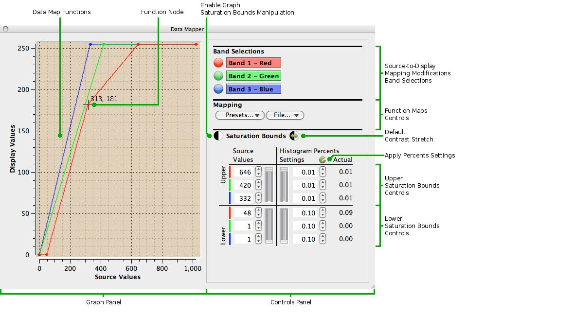
The Data Mapper is divided into a Controls Panel and a Graph Panel. The Data Mapper is a dockable tool. When the tool is located in a side dock area the Graph Panel is not shown; this can result in a more compact application window when only using the Control Panel to manage data mapping values.

The Band Selections control which of the three display bands are affected by all other source-to-display mapping modifications. The Band Selections also apply in the Statistics Source Data tool when manipulating data Bounds on its Histogram.

Clicking on a button toggles the selection of the band for the corresponding display color. The label next to the button indicates which source image data band is mapped to the display color band. If the color name in the label has the first letter underlined that means a keyboard accelerator may be used to toggle the band selection: press the key for the underlined letter while also pressing the Alt key.

The Data Map menu contains a Bands Selections submenu that may be used to select effective bands. This menu also lists the keyboard shortcuts that may be used to toggle band selections.

The Mapping section contains two pop-down menus for controlling the function maps as a whole. Only the mappings for the currently selected bands will be affected by whatever mapping control is used.

The Presets menu lists mapping functions that have been preset within the Data Mapper. These are commonly used functions that are typically applied to reset the mappings for the selected bands to a "standard" state after having explored various alternatives.

The Limited Linear function linearly maps source data between the valid data Limits set in the Source Data Statistics tool. Source values at and below the lower limit are mapped to zero; values at and above the upper limit are mapped to the maximum display value (255). Source values between the limits are mapped from zero to the maximum display value using a linear mapping function. A linear function, as the name implies, appears as a straight line between the lowest and highest values.

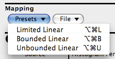
Note that Limited Linear mapping forces the Saturation Bounds of the selected bands to be the same as the valid data Limits.

The Bounded Linear function linearly maps source data between the Saturation Bounds. Source values at and below the lower limit are mapped to zero; values at and above the upper limit are mapped to the maximum display value (255). Source values between the limits are mapped from zero to the maximum display value using a linear mapping function.

The Unbounded Linear function linearly maps source data between the minimum and maximum data values without regard for valid data Limits.

Note that Unbounded Linear mapping forces the Saturation Bounds of the selected bands to the minimum and maximum source data values.

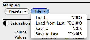
The File menu enables the current data mapping functions to be saved to a file and loaded from a file. The functions may be saved as an image of the Graph or as a set of function Nodes. Function Nodes are saved in a text file in Comma Separated Value (CSV) format. CSV is a standard tabular data format that can be read by other data charting and spreadsheet programs. Data mapping functions may restored from saved Function Nodes files.

HiView's Function Nodes files list the node values following the name (case insensitive) of the display band color to which they apply; each display band name must be on a line by itself. A node is defined by a pair of numbers: the source data value followed by the display data value separated by a comma and/or space (or horizontal tab character); more than one node may be listed on a line. The order of the nodes in the list is not important. When nodes specify the same source data value only the first such node is used. A display band name may occur more than once: All nodes following a display band name, up to the next display band name, are accumulated into a single list for the band. Blank lines are ignored. Characters on a line following a crosshatch ('#') character, and including this character, are ignored as comments.

The Load Data Mapper File dialog is presented, which is used to select a file containing Function Nodes. The filename does not have to have a "csv" extension (though this is usually the case) but it must specify the Function Nodes in HiView's Function Nodes format. The file selection dialog functions like the dialog used to Open an Image File.

When the file has been chosen all Function Nodes found in the file will be applied to the selected bands; all nodes for the selected bands will be replaced with the new nodes and nodes for unselected bands will not be affected.

The last file successfully used to load or save data mapping Function Nodes is remembered. The Load from Last menu item is a shortcut to reload the last file. This might be done after data mapping alternatives have been explored or when the band selections have changed.

The Save Data Mapper File dialog is presented, which is used to select a file where the Function Nodes will be saved. The file selection dialog functions like the dialog used to Save an Image File. The file type selected in the dialog will determine the type of file that is saved. A CSV file type saves all the Function Nodes (regardless of band selections) to a HiView Function Nodes file. Selecting an image file type will result in an image of the Function Graph being saved.

The last file successfully used to load or save data mapping Function Nodes is remembered. The Save to Last menu item is a shortcut to rewrite the the last file with the current Function Nodes.

Note that only Function Nodes files are remembered. When the Function Graph image is saved the file used is not remembered.

Saturation Bounds are a special characteristic of an image data mapping function. Those source data values at the high end of a data mapping function that are all mapped to the maximum display data value are said to be high saturated. Likewise, those source data values at the low end of a data mapping function that are all mapped to display data value zero are said to be low saturated. Source data values between these Saturation Bounds are typically mapped to display data values in some uniform manner; for example source data values might be mapped to display data values that are proportionally equivalent.

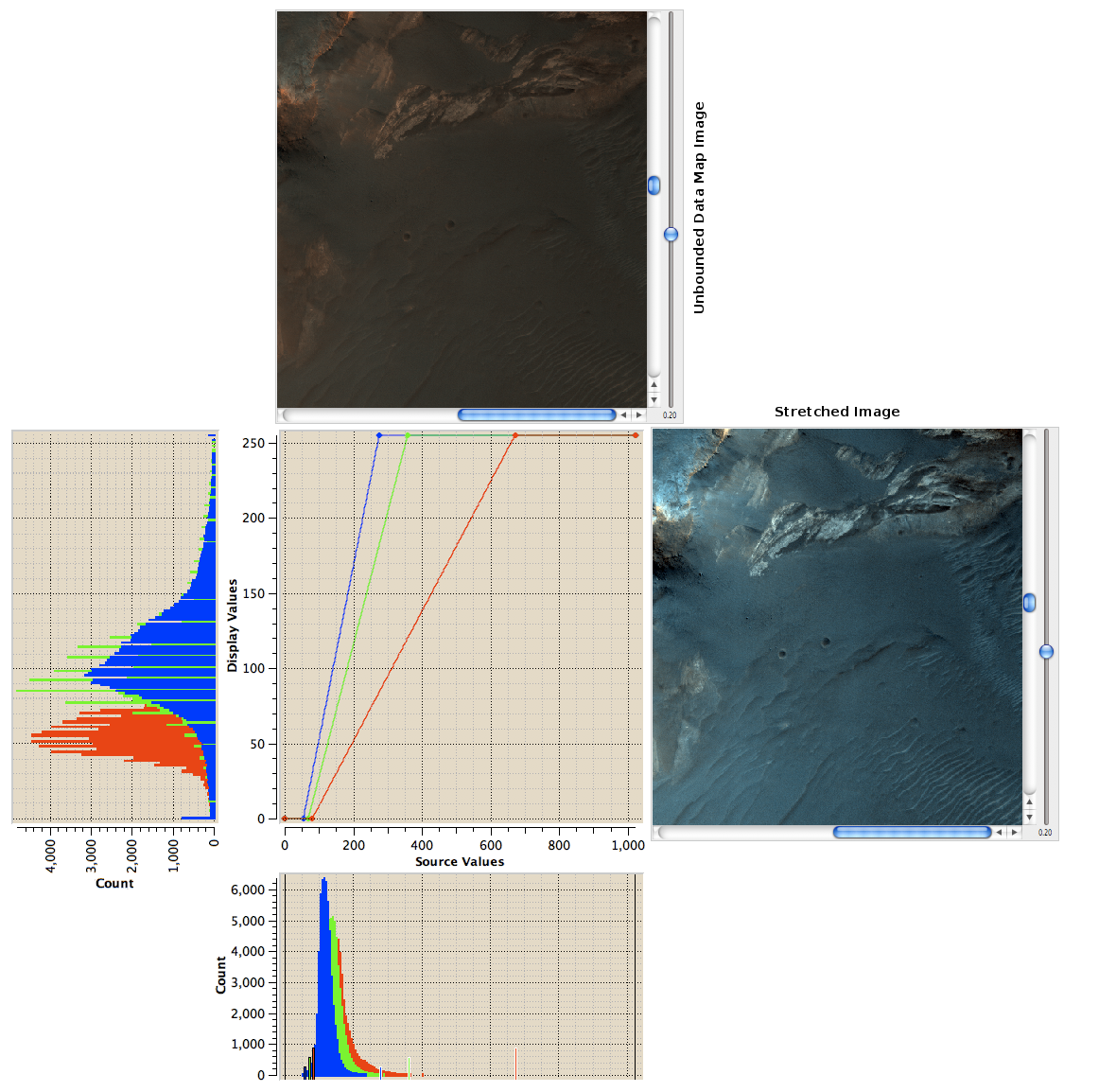
Normally the Saturation Bounds for the data mapping functions are set to the minimum and maximum source data values under the presumption that all source data values are to be displayed with a proportional display data value. However, it is not uncommon for an image to have pixel data values that are not distributed over the full range of possible pixel values. In this case it may be difficult to see detail in the image, or the colors of the image may be perceptually "muddy" or otherwise appear distorted, when all source data pixel values are mapped to their proportional display values. In such cases moving the Saturation Bounds to better correspond to the distribution of pixel values in the source data and remapping the more limited source data range to proportional values over the full range display range is likely to provide significantly enhanced visual fidelity of the source data in the displayed image. This is called a Contrast Stretch.

Contrast stretching can be achieved by interactively manipulating the saturation bounds. A reasonable Contrast Stretch can usually be produced by setting the Saturation Bounds at, or near, the ends of the pixel values distribution range in the source data and linearly mapping the source data between the Saturation Bounds to full range of display data values. Knowing the distribution of source pixel values in the displayed image region is necessary to automatically set appropriate Saturation Bounds for a reasonable Contrast Stretch. The pixel value distribution can be obtained from the Statistics Histograms.

In the example, above, the Unbounded Data Map Image was displayed in the Main Window Display Viewport using mapping functions generated by the Unbounded Linear Presets Mapping. The Stretched Image is the same image region after clicking the Default Contrast Stretch button icon to the right of the "Saturation Bounds" label in the Controls Panel; the Default Contrast Stretch item from the Data Map menu could also be used. At the bottom is the Source Data Histogram, and to the left the Display Data Histogram after applying the Default Contrast Stretch, for the image region. The Data Mapper Graph in the center shows the data mapping functions for each displayed image band with the Saturation Bounds set to Source Values determined from the Source Data Histogram using the Histogram Percents of the default Preferences Default Contrast Stretch settings. After setting the appropriate Saturation Bounds Values the Default Contrast Stretch automatically applies the Bounded Linear data mapping functions which stretch the distribution of Source Values to the distribution of Display Values in the Display Data Histogram. Note that each band of data is stretched differently depending on its distribution of pixel values in the image region. This has produced a "false color" effect in the displayed image and also revealed details and patterns in the source data that are difficult to see otherwise.

After applying the Default Contrast Stretch the image data can be explored further by making additional adjustments to the Saturation Bounds and manipulating data mapping Function Nodes. For example, adding a bend in a data mapping function will effectively apply different contrast stretches to different sections of the function.

The Saturation Bounds can be specified by the Source Values where they occur in the data mapping functions. Controls are provided that report the current Source Values of the Saturation Bounds, and these values may be directly modified to change the corresponding bounds values. Only the controls for selected bands will be enabled. Next to the individual value controls is a slider that will change the bounds of all selected bands to the same value as the slider thumb is dragged. The upper end of the slider is the maximum possible source value and the lower end is zero. Clicking in the slider above or below the thumb will increment the selected values by one in the corresponding direction. Continuing to press on the slider will cause the values to continue to increment.

The Saturation Bounds can be specified as the percentage of the Statistics Histograms for the Source Data that is above, for Upper Saturation Bounds, or below, for Lower Saturation Bounds, the bounds values. For example, at an Upper Histogram Percents Settings of 1.0, one percent of the cumulative Counts - either the entire image region in the Display Viewport, or a subregion selected when the Statistics tool is active - for the selected bands will be at Values greater than or equal to the Upper Source Values. That is, the Histogram Percents determine Saturation Bounds by the amount of Histogram area for the corresponding band above the Upper bounds and below the Lower bounds.

The Histogram Percents Settings have controls that work just like the controls for the Source Values. When the Percent Settings controls are used the corresponding Source Values fields change to indicate the changed Saturation Bounds values, and the Actual Histogram values change to indicate the actual Histogram Percents for the Source Values determined by the Settings. The Upper Source Values are determined from Histogram Percents Settings by finding the highest Values location in the Histogram where the total of the Count values above the location - excluding the Count values above the upper valid data limit - is at least the specified percentage of the total Counts of all valid pixel Values; the Lower Source Values are determined from Histogram Percents Settings similarly. It is quite likely that the Source Values found will not be at locations resulting in the same Histogram Percents specified in the Settings; the Actual Histogram Percents are actual values at the Source Values. Changing the Source Values Settings will affect the Actual Histogram Percents, not the Settings.

The Histogram Percents Settings are only used to determine Saturation Bounds Source Values when the Settings are changed, or when they are specifically applied. The Histogram Percent Settings can be applied by clicking the Apply Percents button icon between the "Settings" and "Actual" column labels in the Saturation Bounds Histogram Percents section of the Controls Panel, or by selecting the Apply Percents Settings item of the Data Map menu. The Histogram Percents Settings are applied - or the Default Contrast Stretch is used, which resets the Settings - for a "training region" in all or part of the Main Window Display Viewport that has been selected to provide data mapping functions that are representative or optimal for viewing the image when it is scrolled to other locations in the Display Viewport. The Actual Histogram Percents will change as the Statistics Measurements Region is changed.

The Histogram Percents Settings values can be set from the Actual values by using the Percents Settings from Actual Data Map menu. Note that because values in the Histogram Percents controls are rounded to two decimal places Applying the Settings obtained from Actual might change the Actual Percents again.

The Graph Panel displays the data mapping functions as plots of the Source Values and the Display Values to which they are mapped. The Graph Panel will not be shown when the Data Mapper is located in a tool dock on either side of the Main Window. Floating the Data Mapper into its own window, by clicking on the little icon in its header bar to the left of the icon with the 'X' (which will close the tool so it is not visible) or using the tool's pop-up menu and selecting the Floating menu item, provides considerable flexibility in sizing the Graph Panel as desired.

The background color of the Graph can be changed by the Canvas Color setting of the Preferences Graphs section.

The Graph Functions are drawn as plot lines on the graph. The Function plots will change to reflect the current data mappings. When the cursor is over the Function plots canvas it will have a small cross hair shape and the position of the cursor in the Graph will be displayed next to the cursor.

Functions may occur at the same location on the plot, in which case the red band function will occur on top of the green band function which will occur on top of the blue band function.

The Functions can be manipulated interactively. When the cursor gets close to a function plot line a small diamond will appear on the plot indicating a potential grab point. The color of the diamond corresponds to the the data mapping band functions that are selected: red, green, or blue for the corresponding single band; cyan, magenta, or yellow for two corresponding bands - cyan is a combination of green and blue, magenta is a combination of red and blue, yellow is a combination of red and green - and white for all three bands. Only those band functions for which band selections are enabled can be manipulated. This is particularly useful when it is desired to manipulate only one or two band functions that are located in the same place on the graph as another function.

The Selection Sensitivity - how close the cursor needs to be to a function plot for a selection point to appear - is controlled by the Selection Sensitivity setting of the Preferences Graphs section.

Clicking on a function plot grab point will cause full-width and full-height yellow positioning lines to appear and a node will be added to the data mapping function at the grab point, if one is not there already.

A data mapping function is defined by its Node values. Mapping function values between the Nodes are linearly interpolated. Each Node of a function mapping is represented on its function plot by a small diamond with the color of the function's band. When a node has been grabbed it may be dragged to any valid new position on the graph and the data mapping function will change accordingly and the image displayed in the Main Window Display Viewport will change along with the changes to the data mapping function.

Since the data mapping functions are monotonic - i.e. a Source Value may only be mapped to one Display Value - a node may not be moved to a position that overlaps any adjacent node of the same band function. However, if a node is dragged over an adjacent node of the same band function the adjacent node is replaced by the node being dragged.

There will always be Nodes at the minimum (zero) and maximum Source Values. These anchor Nodes may be dragged to a new vertical position at the same Source Value. But if they are dragged horizontally into the Graph area a new node is automatically added to the function adjacent to the anchor node; dragging out the Graph area has no effect, though the node position will still be moved vertically if the cursor is moved vertically.

There are two other special nodes for each data mapping function: Nodes for the Saturation Bounds. These are the nodes adjacent to, or at, the end point anchor nodes. When an anchor node is not located at the minimum or maximum Display value position, the anchor node is the node for the Saturation Bound of its function. Otherwise the node adjacent to the anchor node that is also at the minimum or maximum Display Value position of its adjacent anchor node is the Saturation Bound node. Saturation Bounds nodes may be manipulated like any other node. If they are dragged away from the minimum or maximum position of the adjacent anchor node they are no longer a Saturation Bound node and the Saturation Bound node will revert to the anchor node. Conversely, if a node adjacent to an anchor node at the minimum or maximum Display Value position is dragged to the same Display Value position it becomes the Saturation Bound node..

To make manipulating Saturation Bounds nodes more straightforward, the gray button to the left of the Saturation Bounds section label in the Controls Panel may be clicked to enable only manipulating Saturation Bounds Nodes in the Graph. The icon will change to half black and half white to indicate that Saturation Bounds manipulation mode is in effect, and the cursor over the Graph area will change to a vertical line with a horizontal double-header arrow at the cursor position. When the horizontal cursor position gets within the selection distance of a Saturation Bounds node the double-headed arrow will change to a vertical bar with pointer in the inward direction of the Graph relative to the Saturation Bound node; i.e. the pointer will be directed to the right for a Lower Bound node, and to the left for an Upper Bound node. In addition, the color of the cursor will be the color of the bands for the functions that are selected. The color is the same as for selecting other Nodes, and the possible selections are also controlled by the current band selections. Clicking and dragging the cursor will relocate the selected Saturation Bounds Nodes.

1.4    2011/09/08 06:09:44