- Measure
- Analyze Particles...
- Summarize
- Clear Results
- Set Measurements...
- Set Scale...
- Calibrate...
- Histogram
- Plot Profile
- Show LUT
- Gels>
- Tools>
Based on the selection type, calculates and displays either area statistics or line lengths. Area statistics are calculated if there is no selection or if a subregion of the image has been selected using one of the first four tools in the tool bar. Calculates line length if a line selection has been created using one of the three line selection tools. Use the Analyze/Measurement Options to specify what area statistics are recorded.
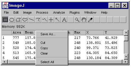
To export the measurements as a tab-delimited text file, use File/Save As/Measurements or select one or more lines (shift-click to extend the selection) and use Edit/Copy (C) or Edit/Cut (X). You can also save measurements by right-clicking (control-clicking on a Macintosh) in the worksheet and selecting Save As or Copy from the popup menu.
The width of the worksheet columns can be adjusted by clicking on and dragging the vertical lines that separate the column headings.
Analyze Particles...
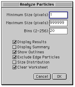
Particles smaller than Minimum Size or larger than Maximum Size are ignored. Bins is the number of bins used for the particle size distribution histogram. Check Display results to have the measurements for each particle displayed in the ImageJ worksheet. Check Show Outlines to display a window containing numbered outlines of the measured particles. Check Exclude Edge Particles to ignore particles touching the edge of the image. Check Size Distribution to display a particle size distribution histogram. Check Clear Worksheet to erase any previous measurement results.
Summarize Clear Results Set Measurements...
Mean Gray Value - Average gray value within the selection. This is the sum of the gray values of all the pixels in the selection divided by the number of pixels. Reported in calibrated units (e.g., optical density) if Analyze/Calibrate was used to calibrate the image.
Standard Deviation- Standard deviation of the gray values used to generate the mean gray value.
Modal Gray Value - Most frequently occurring gray value within the selection. Corresponds to the highest peak in the histogram.
Min & Max Gray Level - Minimum and maximum gray values within the selection.
Centroid - The center point of the selection. This is the average of the x and y coordinates of all of the pixels in the selection.
Center of Mass - This is the brightness-weighted average of the x and y coordinates all pixels in the selection.
Perimeter - The length of the outside boundary of the selection.
Bounding Rectangle - The smallest rectangle enclosing the selection. Uses the headings BX, BY, Width and Height, where BX and BY are the coordinates of the upper left corner of the rectangle.
Fit Ellipse - Fit an ellipse to the selection. Uses the headings Major, Minor and Angle. Major and Minor are the primary and seconday axis of the best fitting ellipse. Angle is the angle between the primary axis and a line parallel to the x-axis of the image.
Limit to Threshold - If checked, only thresholded pixels are included in measurement calculations. Use Image/Adjust/Threshold to set the threshold limits.
Display Row Labels - If checked, the image name and slice number (for stacks) are recoded in the first column of the results table.
Decimal Places - This is the number of digits to the right of the decimal point in real numbers displayed in the results table and in histogram windows.
Set Scale...
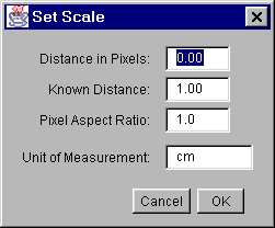
Set Distance in Pixels to zero to revert to pixel measurements.
Setting Pixel Aspect Ratio to a value other than 1.0 enables support for different horizontal and vertical spatial scales, for example 100 pixels/cm horizontally and 95 pixels/cm vertically. To set the pixel aspect ratio, measure the width and height (in pixels) of a digitized object with a known 1:1 aspect ratio. Enter the measured width (in pixels) in Distance in Pixels. Enter the known width in Known Distance. Then calculate the aspect ratio by dividing the width by the height and enter it in Pixel Aspect Ratio.
Calibrate...
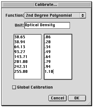
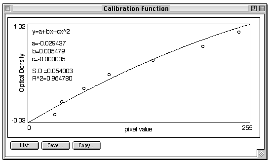
When finished making the measurements, select Analyze/Calibrate to display the Calibrate dialog box. To calibrate the image, enter the known standard values in the right column, select a curve fitting method from the popup menu, enter the unit of measurement, and click OK. ImageJ will then display the calibration function.
If the calibration function is not satisfactory, bring up the Calibrate dialog box again and select a different curve fitting method.
Rodbard is a four parameter general curve fit function proposed by David Rodbard at NIH. The form of the equation is:
Histogram
With RGB color images, the histogram is of the combined red, green and blue channels. With 16-bit images, the range of gray values between Min and Max is divided into 256 bins. With 32-bit images, the number of bins can be specified in the Edit/Options/Miscellaneous dialog box.
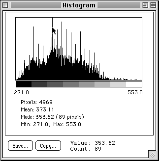
Use the Save or Copy buttons to save the histogram data, formatted as 256 lines each containing a single number. Value:, which changes as you move the cursor, is the grayscale value corresponding to the x-axis cursor position and Count: is the number of pixels that have that value.
Plot Profile
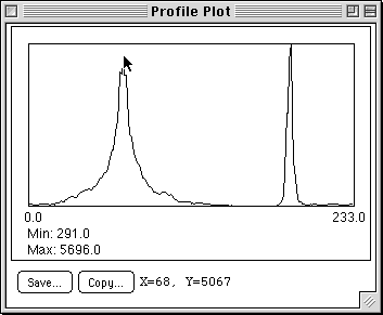
For rectangular selections, displays a "column average plot", where the x-axis represents the horizontal distance through the selection and the y-axis the vertically averaged pixel intensity. To average horizontally, hold down the alt key. Use the Save or Copy buttons to save the profile data, formatted as a sequence of lines each containing a single number.
Show LUT
Gels>
Here is what you need to do to analyse a 1-D gel:
Tools> Save XY Coordinates... Box Count... Analyze Line Graph ROI Manager (ImageJ 1.25 and newer)
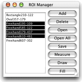
Click Add to add the current ROI to the list. Click Delete to delete the selected ROIs from the list. Click Open to open an ROI file and add it to the list. Click Open All to open all the ROI files in a folder and add them to the list. Click Save to save the selected ROIs as files. Click Measure to measure the selected ROIs. With a stack, a dialog box allows the user to choose between measuring all of the images in the stack or only the current slice. Click Draw to draw outlines of the selected ROIs using the current foreground color and line width. Click Fill to fill the selected ROIs with the current foreground color. Click in the Image/Colors window to set the foreground color. Use Edit/Options/Line Width to set the line width.
This command counts and measures objects in binary or thresholded images. It works by scanning the image or selection until it finds the edge of an object. It then outlines the object using the wand tool, measures it using the Measure command, fills it to make it invisible, then resumes scanning until it reaches the end of the image or selection. Press the esc key to abort this process.
Use Image/Adjust/Threshold to threshold an image.
For each column in the results table, calculates and displays the mean, standard deviation, minimum and maximum of the values in that column.
Erases the results table and resets the measurement counter.
Use this dialog box to specify which measurements are recorded by Analyze/Measure and Analyze/Analyze Particles.
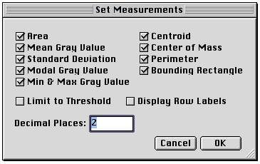
Area - Area of selection in square pixels. Area is in calibrated units, such as square millimeters, if Analyze/Set Scale was used to spatially calibrate the image.
Use this dialog to define the spatial scale of the active image so measurement results can be presented in calibrated units, such as millimeters. Before using this command, use the straight line selection tool to make a line selection that corresponds to known distance. Then, bring up the Set Scale dialog, enter the known distance and unit of measurement, then click OK. ImageJ will have automatically filled in the Distance in Pixels field based on the length of the line selection.
Use this dialog box to calibrate an image to a set of density standards, for example radioactive isotope standards or a calibrated optical density step tablet. Before using this command, use Analyze/Clear Results to reset the measurement counter and use one of the selection tools and Analyze/Measure to record the mean gray value of each of the standards.
y = a + (a - d) / (1 + (x/c)^b)
Selecting Uncalibrated OD from the popup menu causes ImageJ to convert gray values to uncalibrated optical density values using the function
Uncalibrated OD = log10(255 / PixelValue)
You do not need to measure OD standards or enter known OD values to enable this feature.
Calculates and displays a histogram of the distribution of gray values in the active image or selection. The x-axis represents the possible gray values and the y-axis shows the number of pixels found for each gray value. The total pixel count is also calculated and displayed, as well as the mean, modal, minimum and maximum gray value.
Displays a two-dimensional graph of the intensities of pixels along a line within the image. The x-axis represents distance along the line and the y-axis is the pixel intensity.
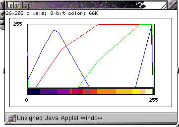
Displays a plot of the active image's lookup table. The lookup table, or color table, describes the color that is displayed for each of the 256 possible pixel values. A bar under the plot displays the color representation of the pixel values. Note that RGB color images do not use a lookup table.
Use the commands in this submenu to analyze one-dimensional electrophoretic gels using ImageJ's built in Gel Analyzer plugin. This plugin is similar to
the Gel Plotting Macros
distributed with NIH Image. Both use a simple graphical method that involves generating lane profile plots, drawing lines to enclose peaks of interest, and then measuring peak areas using the wand tool.
This submenu provides access to various image analysis plugins.
| Plugins Menu
| Contents
| Home |
Writes to a text file the XY coordinates and pixel value of all non-background pixels in the active image. For grayscale images, writes three values per line (x, y, and value), separated by spaces. For RGB images, writes five values per line (x, y, red, green and blue).
Counts the number of boxes of an increasing size needed to cover a one pixel binary object boundary. The box size and the number of boxes necessary to cover the boundary are plotted on a log-log plot and the fractal dimension determined from the slope, i.e. D=-slope. For more information, see the "Fractal_Box_Counter.java" source file.
ImageJ can be used to recover numeric coordinate data from scanned line graphs using the following procedure. Steps 1-6 are not necessary for binary (black and white) graphs. For practice, use the File/Samples/Line Graph sample image.
The ROI (Region of Interest) Manager is a tool for working with multiple area selections.
