Oleg Abramov
Planetary Image Research Laboratory
Abstract
The Mars Orbiter Laser Altimeter (MOLA) instrument on the Mars Global Surveyor (MGS) spacecraft has returned a large amount of data on the topography of Mars. It is possible to generate high-resolution Digital Elevation Models (DEMs) from this data by employing data interpolation techniques. Four interpolation algorithms were selected to be tested on MOLA data: Delaunay-based linear interpolation, splining, nearest neighbor (or Inverse Distance Weighting), and natural neighbor. These methods were applied to the MOLA data of Korolev crater (a large crater in the north polar region of Mars) for qualitative analysis. In addition, a known DEM of a part of Iceland was used for both qualitative and quantitative testing. The quantitative testing was conducted by simulating MOLA data acquisition, interpolating that data, and then calculating the mean absolute error (MAE) between the interpolated DEM to the original DEM. Also, execution speeds were measured for the four algorithms. The natural neighbor method appears to be superior both quantitatively and qualitatively to other methods tested, but is relatively slow computationally.
Introduction
The Mars Orbiter Laser Altimeter (MOLA) instrument on the Mars Global Surveyor (MGS) spacecraft has been collecting topography data from the orbit of Mars over the last several years. MOLA fires 1064 nm laser pulses at the surface at a rate of about 10 per second (1). When the laser strikes the surface, some fraction of the laser energy is backscattered in the direction of the spacecraft, and range is calculated from round-trip travel time. At the time of writing, over 600 million data points have been collected (2). The MGS spacecraft is in a near-polar orbit with an inclination of 93° (3), so the spatial resolution of the MOLA data increases with latitude.
Currently, global topography datasets are the main source of the digital elevation models (DEMs) of localized regions on Mars. These datasets are called Experiment Gridded Data Records (EGDRs), and are constructed by taking the median observed topography within a specified degree area. At this time, the highest resolution EGDR is 1/32 degrees per pixel (4).
However, using data interpolation techniques instead of calculating median elevations can result in higher-resolution DEMs. On the other hand, it should be noted that most common interpolation algorithms were formulated to work with randomly distributed data (5), and give visible artifacts when applied to MOLA tracks. The data points within each MOLA track are regularly spaced, and the tracks themselves are either almost parallel to each other or intersect each other at a latitude-dependant angle. The challenge is to find an algorithm that minimizes visible artifacts and is quantitatively accurate at the same time.
The goal of this project was to test several common interpolation techniques, namely Delaunay-based linear interpolation, splining, nearest neighbor (also called Inverse Distance Weighting), and natural neighbor. These techniques were applied to MOLA data for qualitative testing. In addition, quantitative testing of simulated MOLA data obtained from a known DEM was performed.
Methods
1. Acquisition of MOLA altimetry data
MOLA data was obtained from PEDR (Precision Experiment Data Record) files on CD volumes up to MGSL0033. The pedr2tab program was used to extract data within specified latitude and longitude constraints, and to convert it from binary to ASCII format. It is important to note, however, that pedr2tab outputs all MOLA frames found within a given latitude and longitude range, and some data points in these frames often lie beyond the desired coordinate range.
2. Data processing
The edit_PEDR_table.pl script is used to remove the data points that fall beyond the desired spatial range. The trim_PEDR_table.pl script is then executed to put the data into a standard xyz format. The results are in the following format: "longitude(East) latitude(areocentric) topography."
3. Raw data visualization (optional)
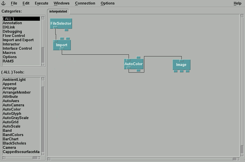
Raw MOLA data from step 2 can be quickly visualized in OpenDX. A mola.general file is created to describe the format of the data and the number of data points. The "more MOLAdatafile | wc -l" command can be used to determine the number of data points in the dataset.
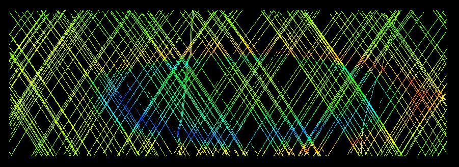
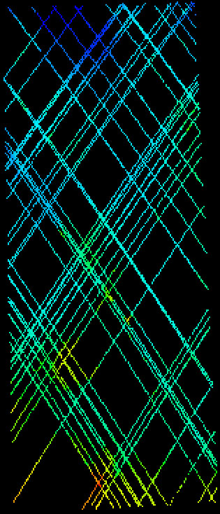
For the initial visualization of the data, the show_altimetry.net program is executed. The typical output is shown in Fig 1.
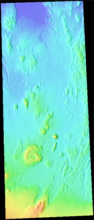
Figure 1. MOLA tracks for the Korolev crater. Elevation is color-coded, with red representing
high altitudes and blue representing low altitudes. The map projection is simple cylindrical.
4. Interpolation for missing data points
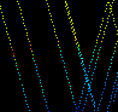
Figure 2. Close-up view of the MOLA tracks shown in Fig.1. Individual data points are visible.
4a. Linear Interpolation
Linear interpolation performs a Delaunay triangulation of a planar set of data points. After the irregularly gridded data points have been triangulated, the surface values are interpolated to a regular grid (6).
In IDL, these procedures are carried out by TRIANGULATE and TRIGRID, respectively. The sequence of IDL commands is as follows:
openr, 1, 'xyz_elevation.dat'
xyz_array = fltarr( 3, [number of data points] )
readf, 1, array
close, 1
x = xyz_array( 0, *, * )
y = xyz_array( 1, *, * )
z = xyz_array( 2, *, * )
triangulate, x, y, tr
interpolated_elevation = trigrid( x, y, z, tr [,options] )
openw, 1, 'interpolated_elevation.dat'
printf, 1, interpolated_elevation
close, 1
The options for TRIGRID can be used to specify the size of the output grid. The output is in the form of a column-major elevation grid, which can be visualized using the SURFACE command or imported into OpenDX.
4b. Splining
Splining is a curve fitting method, which fits a least-cost mathematical function through observed data points (7). Physically, it is similar to fitting a thin elastic sheet through the given points.
The surface program included in the Generic Mapping Tools (GMT) package was used for the splining interpolation. The following command-line parameters were used: surface xyz_elevation.dat -R[min/max coordinates of the input data] -Gxyz_elevation.out -I[output grid increment] -N1000000
These parameters result in 106 maximum iterations in each cycle, and give a minimum curvature solution. The GMT grd2xyz command is used to convert the output file to an ASCII xyz file, which can then be imported into IDL or OpenDX for visualization.
4c. Nearest Neighbor
In general, for every point of the output grid, a weighted average of n closest data points is performed. The weighting factor used most frequently is 1/ri2, where ri is the distance from the point being interpolated to the data point i (8).
While a nearest neighbor routine is available in the Autogrid module of OpenDX, it does not allow the user to rigorously define an output grid. There is also a nearneighbor program available in the GMT package; however, it performs a sector-based neighbor search, which does not work well for MOLA data if a large n is used.
As a result, a simple nearest-neighbor procedure was implemented in C. A value of n = 50 was used for all tests. The output of the program is an ASCII xyz file.
4d. Natural Neighbor
The natural neighbor interpolation method has some features in common with linear and nearest neighbor techniques. In particular, it involves Delaunay triangulation and a weighted average, but it successfully avoids some of the problems of these techniques. It differs primarily by the method of neighbor selection and the fact that weights are based on proportionate areas, rather than distances (9).
Natgrid is a natural neighbor interpolation package which is part of the ngmath library distributed with NCAR Graphics. Single - precision C programs natgrid_linear.c and natgrid_nonlinear.c pre-process the data and feed it to the natgrid package. For this evaluation, the linear version was used. The sample command line used to compile and link the above programs is gcc natgrid_linear.c -L/$HOME/NCAR/lib -I/$HOME/NCAR/include -lncarg -lncarg_gks -lncarg_c -lngmath -lF77 -lM77 -lsunmath -lm -lX1 -O3. The output is a row-major elevation grid.
5. Qualitative analysis
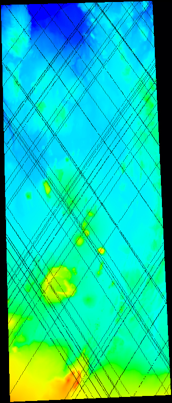
The above techniques were used to interpolate MOLA data of the Korolev crater region (161.00 - 167.00E, 72 - 74N), the Milankovic crater region (211.00 - 216.00E, 53.50 - 55.70N), and a random location (95.00 - 96.00E, 59.00 - 60.00N). The interpolated DEMs generated using the above methods were imported into OpenDX and visually compared.
6. Quantitative analysis
For quantitative analysis, a DEM of a part of Iceland (15°45' - 17°15' W, 64°35' - 66°10' N) was used. The general concept is to sample data from it simulating the way MOLA acquires data, interpolate that data, and then numerically compare the interpolated DEM to the original DEM. (Fig. 3)
 2.
2. 
For step 1 in Figure 3, the coordinates for the Korolev crater MOLA data were rounded to the nearest thousanth by the round_MOLA_data.pl script, and then scaled to x:1-6000, y:1-2000 by the 161_72scale.pl script. The edit_MOLA_table.pl script was then used to grab MOLA points in the range x:1-836, y:1-1967, which is the size of the Iceland DEM.
For step 2, get_elevation.pl script was used to assign elevations to the MOLA points. These points were then used as input for several interpolation techniques. The resulting interpolated DEMs were then compared to the original DEM on a point-by point basis, and the mean absolute error (MAE) was calculated by the compare_DEMs.pl script.
Results
1. Qualitative results
1a. Korolev crater
 |  |
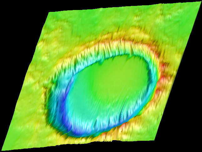 | 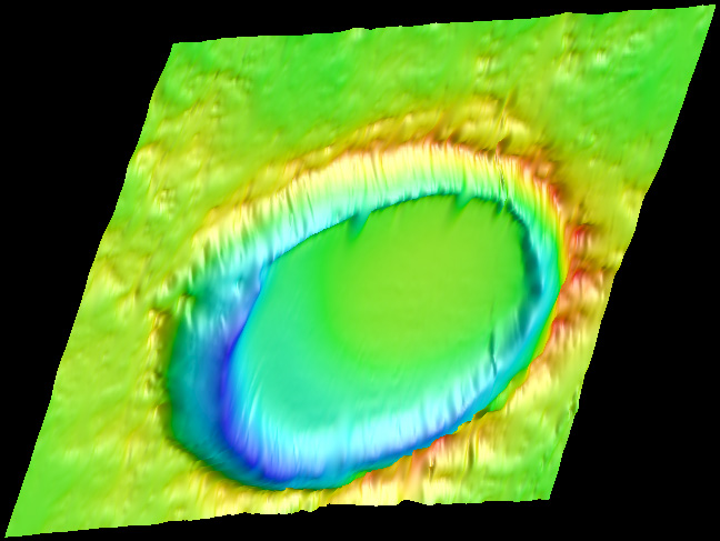 |
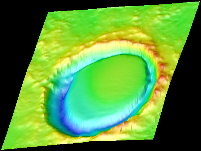
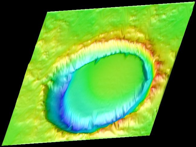
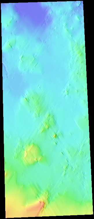
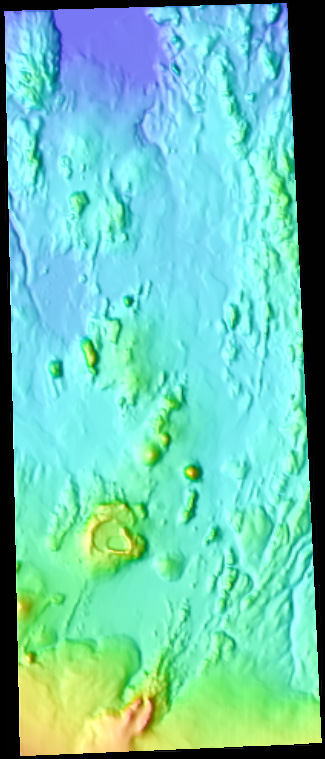
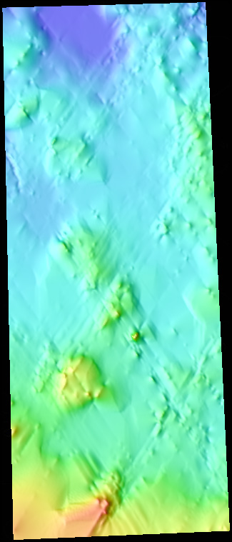
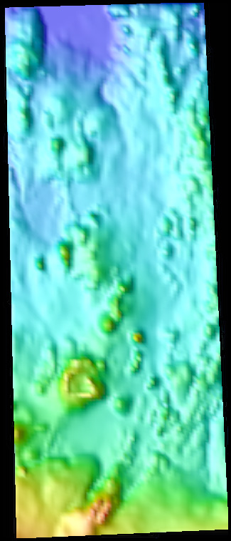
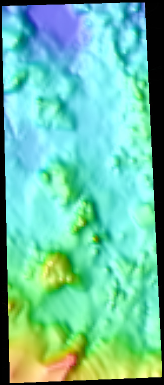
Figure 4. Relief-shaded topography generated by the four interpolations methods that were applied
to the Korolev crater MOLA data (161.00 E - 167.00 E, 72.00 N - 74.00 N). The output grid
is 600 x 200; the aspect ratio was changed to make the crater appear circular. Clockwise from top
left: natural neighbor, linear, nearest neighbor, splining. The mean crater diameter is 80 km (10).
1b. Iceland DEM
1.  | 2. 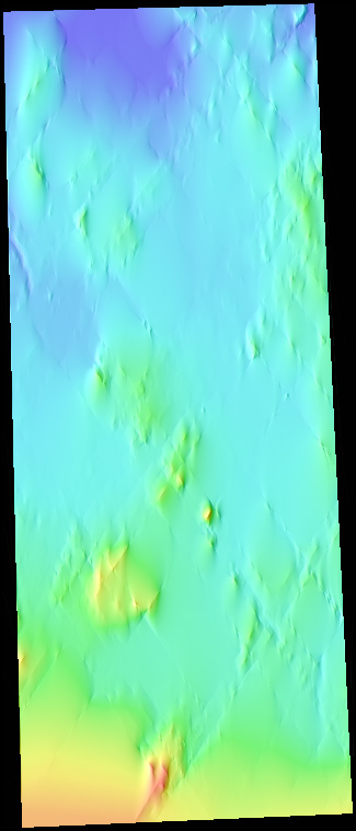 | 3.  |
4.  | 5. 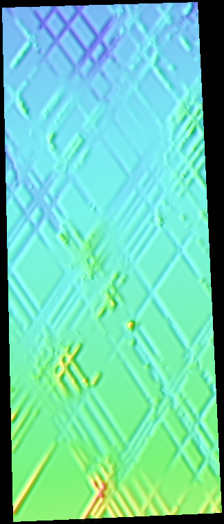 | 2 - Natural neighbor linear interpolation 3 - Linear interpolation 4 - Nearest neighbor interpolation (n = 50) 5 - Splining interpolation (max. iterations per cycle = 106) |
Figure 5. Full-resolution (836 x 1967) interpolation of the original DEM.
1.  | 2. 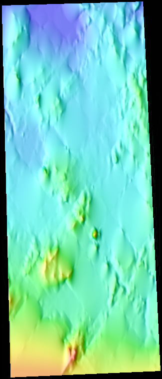 | 3. 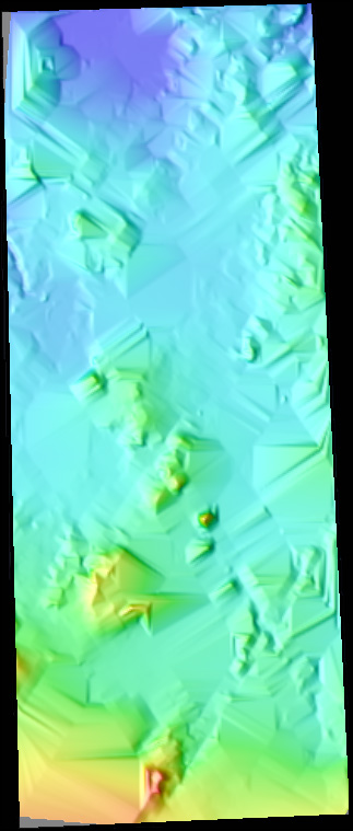 |
4.  | 5. 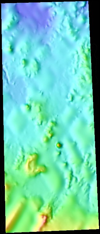 | resampled to 209 x 492 2 - Natural neighbor linear interpolation 3 - Linear interpolation 4 - Nearest neighbor interpolation (n = 50) 5 - Splining interpolation (max. iterations per cycle = 106) |
Figure 6. Medium resolution (209 x 492) interpolation of the original DEM.
1.  | 2. 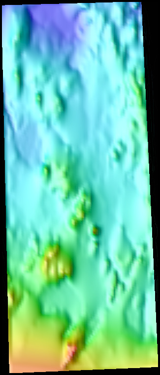 | 3. 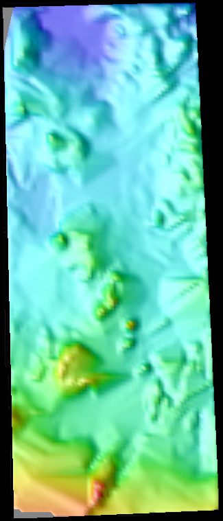 |
4.  | 5. 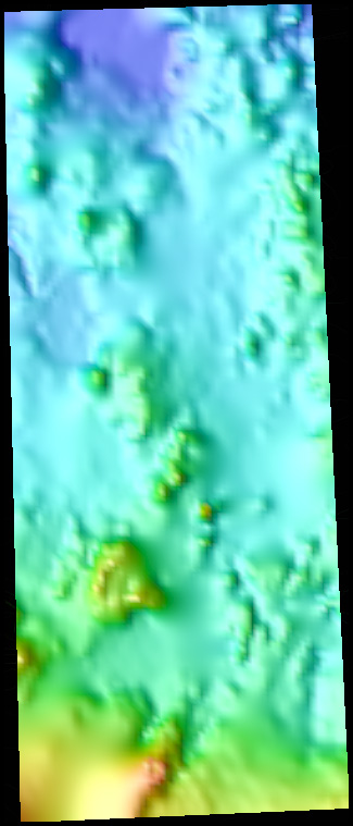 | resampled to 69 x 162 2 - Natural neighbor linear interpolation 3 - Linear interpolation 4 - Nearest neighbor interpolation (n = 50) 5 - Splining interpolation (max. iterations per cycle = 106) |
Figure 7. Low resolution (69 x 162) interpolation of the original DEM
2. Quantitative results
| Natural Neighbor | ||||||
| Linear | ||||||
| Nearest Neighbor | ||||||
| Splining | ||||||
Table I. Summary of the quantitative analysis of interpolation techniques. All values are in meters.
For the nearest neighbor technique, the number of nearest neighbors (n) was 50. For splining, 106
maximum iterations per cycle were used.
Execution Time | |
| Natural Neighbor | 02 hours 08 minutes 47.53 seconds |
| Linear | 00 hours 00 minutes 05.70 seconds |
| Nearest Neighbor | 11 hours 09 minutes 11.58 seconds |
| Splining | 00 hours 00 minutes 30.55 seconds |
Table 2. Execution times for the interpolation of the Korolev crater MOLA dataset (80732 data
points) on a 440 Mhz UltraSPARC IIi processor. The output grid is 600 x 200. For the nearest
neighbor technique, the number of nearest neighbors (n) was 50. For splining, 106 maximum
iterations per cycle were used.
Discussion
The results indicate that the natural neighbor algorithm consistently outperformed other techniques both quantitatively and qualitatively. The Korolev crater qualitative results demonstrate that the natural neighbor algorithm can be readily applied to MOLA data to produce high quality interpolations. The DEM generated by the natural neighbor method has fewer interpolation artifacts, in both number and severity, compared to the other methods.
For the full resolution (836 x 1967) interpolation of the Iceland DEM, the natural neighbor algorithm produced a realistic DEM with the fewest interpolation artifacts. It is also very promising that the overall lowest mean absolute error was achieved for the natural neighbor full resolution interpolation. The splining algorithm clearly didn't work well for this resolution, and other methods had pronounced artifacts.
For the medium resolution (209 x 492) interpolation, splining appears mostly artifact-free, but is highly inaccurate when analyzed numerically. Both linear and nearest-neighbor methods result in a large number of visible artifacts and are quantitatively inferior.
The only exception are the low resolution (69x 162) interpolation results, which show a similar mean absolute error for all four algorithms and, with the exception of linear interpolation, have a roughly similar visual appearance. However, it was anticipated for different interpolation methods to manifest their differences the most at high resolutions, and converge at low resolutions, so these results are not unexpected.
The processing speed tests indicate a large performance gap, with the linear and splining methods being by far the fastest, and natural neighbor and nearest neighbor being the slowest. On the other hand, the execution time for the natural neighbor algorithm is still quite reasonable, and should suffice for most applications. Given this method's quantitative and qualitative advantages, it should be used unless processing time is a serious concern.
Conclusion
While further quantitative testing is desirable, it is clear that the natural neighbor algorithm yields excellent results when applied to MOLA data. Additional investigation in this area should include testing of the natural neighbor algorithm on other known DEMs and possibly combining it with the median observed topography technique. The current results indicate that natural neighbor should be the algorithm of choice when accuracy and appearance are required, and splining can be used as a quick first-order interpolation technique. Also, better interpolations than those presented here are now possible with additional MOLA data. With the recently released MOLA datasets 34-54, higher resolutions and better quality is possible.
References
1) Zuber, M.T., D.E. Smith, S.C. Solomon, D.O. Muhleman, J.W. Head, J.B. Garvin, J.B. Abshire, and J.L. Bufton 1992. The Mars Observer Laser Altimeter investigation, J. Geophys. Res. 97, 7781-7798.
2) MOLA shot counter, located at http://sebago.mit.edu/shots/
3) Albee, A.L., F.D. Palluconi, and R.E. Arvidson 1998. Mars Global Surveyor mission: overview and status. Science 279, 1671 - 1672.
4) Smith, D.E., M.T. Zuber, H.V. Frey, J.B. Garvin, J.W. Head, D.O. Muhleman, G.H. Pettengill, R.J. Phillips, S.C. Solomon, H.J. Zwally, W.B. Banerdt, T.C. Duxbury, M.P. Golombek, F.G. Lemoine, G.A. Neumann, D.D. Rowlands, O. Aharonson, P.G. Ford, A.B. Ivanov, P.J. McGovern, J.B.Abshire, R.S. Afzal, and X. Sun, 2001. Mars Orbiter Laser Altimeter (MOLA): Experiment summary after the first year of global mapping of Mars, J. Geophys. Res., in press.
5) Watson, D.F., 1992. CONTOURING: A guide to the analysis and display of spatial data, Pergamon Press.
6) Research Systems, Inc., 2000. IDL reference guide.
7) Hutchinson, M.F., and P.E. Gessler, 1994. Splines - more than just a smooth interpolator, Geoderma, 62, 45-67.
8) Eckstein, B.A., 1989, Evaluation of spline and weighted average interpolation algorithms, Computers & Geosciences 15,79-94.
9) Sibson, R., 1981 A Brief Description of Natural Neighbor Interpolation, in Interpreting Multivariate Data, ed. by V. Barnett, John Wiley & Sons, New York
10) Garvin, J.B., S. E. H. Sakimoto, J. J. Frawley, C. Schnetzler 2000. North polar region craterforms on Mars. Icarus 144, 329-352.